I recently completed a comprehensive study of database design, covering everything from logical modeling to physical implementation. Database design is a critical phase in systems development where we transform conceptual data requirements into actual database structures that applications can use. This process involves two major steps: creating a logical database model and then designing the physical database implementation.
Understanding the Relational Database Model
The relational database model forms the foundation of most modern database systems. In this model, data is represented as a set of related tables, called relations. Each relation is a two-dimensional structure with named columns and rows. What distinguishes a proper relation from a simple table is a set of specific properties that must be satisfied.
A relation must have entries in cells that are simple, meaning no cell can contain multiple values or nested structures. All entries in a column must come from the same set of values, establishing what's known as a domain for that column. Each row must be unique, which is guaranteed by having a nonempty primary key value. The sequence of columns can be interchanged without changing the meaning of the relation, and rows can be stored in any sequence without affecting the logical structure.

The primary key is an attribute or combination of attributes whose value is unique across all occurrences of a relation. This uniqueness is what allows us to identify individual rows and establish relationships between tables. The primary key must satisfy two conditions: it must uniquely identify every row in the relation, and it should be nonredundant, meaning no attribute in the key can be removed without losing the uniqueness property.
Functional Dependencies and Normalization
Functional dependency is a constraint between two attributes where the value of one attribute determines the value of another attribute. We represent this relationship as A → B, meaning attribute B is functionally dependent on attribute A. For every valid value of A, that value uniquely determines the value of B. Understanding functional dependencies is essential because they form the basis for normalization rules.

Normalization is the process of converting complex data structures into simple, stable data structures. The goal is to create well-structured relations that contain minimum redundancy and allow users to insert, modify, and delete rows without errors or inconsistencies. Normalization follows a progression through normal forms, each addressing specific types of problems.
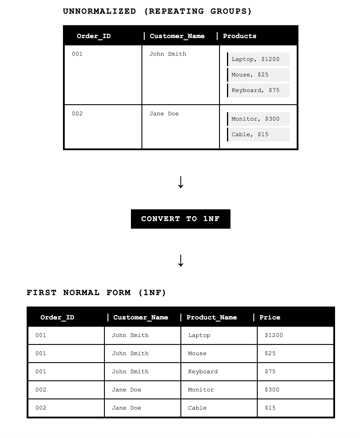
First Normal Form (1NF)
First normal form requires that a relation has no multivalued attributes and that all rows are unique. A multivalued attribute is one that can have multiple values for a single entity instance. For example, if we tried to store multiple phone numbers in a single Phone_Numbers column, we would violate first normal form. The solution is to either create separate columns for each phone number or, more commonly, create a separate related table for phone numbers.
Second Normal Form (2NF)
Second normal form addresses situations where a relation has a composite primary key made up of multiple attributes. A relation is in second normal form if every nonprimary key attribute is functionally dependent on the whole primary key, not just part of it. This is called full functional dependency.
Consider a relation ORDER_LINE(Order_Number, Product_ID, Product_Description, Quantity_Ordered). Here, the primary key is the combination of Order_Number and Product_ID. However, Product_Description depends only on Product_ID, not on the full composite key. This creates a partial dependency.

To convert this to second normal form, we decompose the relation using the determinants as primary keys. The determinant is the attribute that determines other attributes. In this case, we create two relations:
ORDER_LINE(Order_Number, Product_ID, Quantity_Ordered)
PRODUCT(Product_ID, Product_Description)
This eliminates the partial dependency because now Product_Description depends on the full primary key of the PRODUCT relation.
Third Normal Form (3NF)
Third normal form eliminates transitive dependencies between nonprimary key attributes. A transitive dependency occurs when one nonprimary key attribute determines another nonprimary key attribute. A relation is in third normal form when it is in second normal form and has no functional dependencies between nonprimary key attributes.
Consider the relation SALES(Customer_ID, Customer_Name, Salesperson, Region). The primary key is Customer_ID. However, if each salesperson works in only one region, then we have a transitive dependency: Customer_ID → Salesperson → Region.
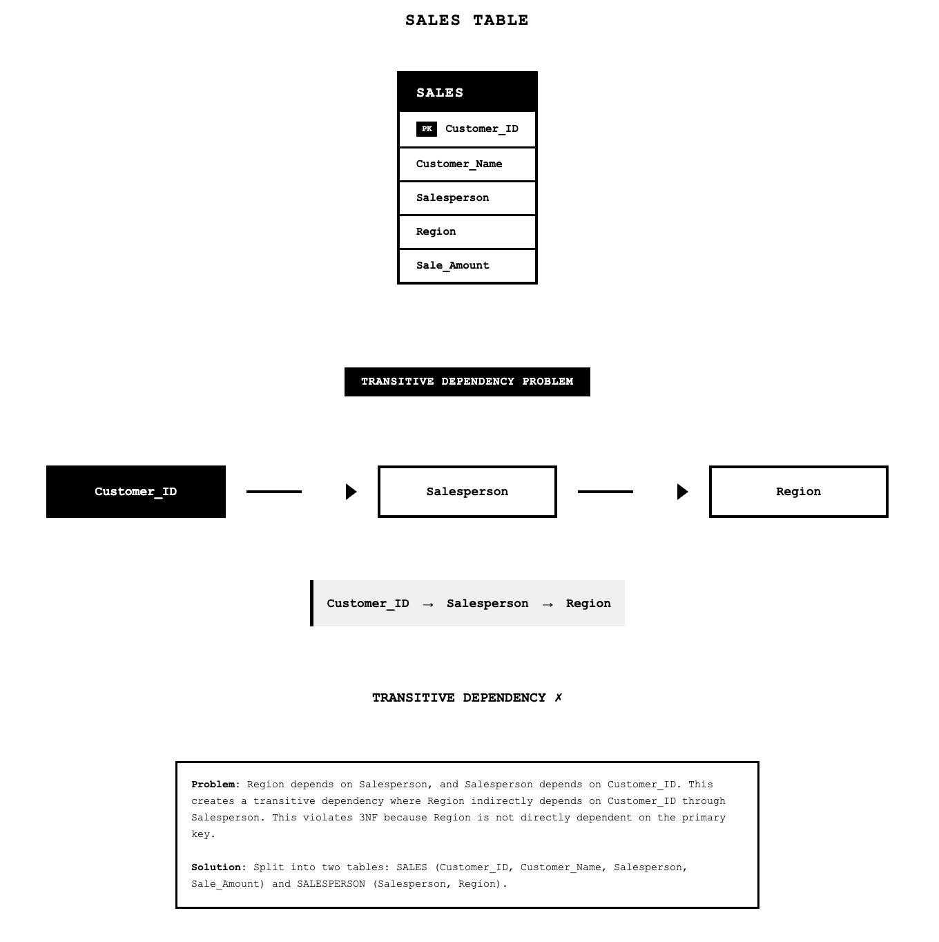
To convert this to third normal form, we split the relation:
SALES1(Customer_ID, Customer_Name, Salesperson)
SPERSON(Salesperson, Region)
The principle behind normalization can be summarized as "the key, the whole key, and nothing but the key," meaning every nonprimary key attribute should depend on the primary key, the complete primary key, and only the primary key.
Transforming E-R Diagrams into Relations
The transformation from entity-relationship diagrams to normalized relations follows systematic procedures that depend on the type of entity or relationship being transformed. Each structure in an E-R diagram has a corresponding relational representation.
Representing Entities
Each regular entity in an E-R diagram becomes a relation. The identifier of the entity type becomes the primary key of the corresponding relation. All attributes of the entity become columns in the table. For example, a CUSTOMER entity with attributes Customer_ID, Name, Address, and Discount becomes the relation CUSTOMER(Customer_ID, Name, Address, Discount).

Representing Binary 1:N Relationships
Binary one-to-many relationships are represented by adding the primary key from the entity on the "one" side of the relationship as a foreign key in the relation on the "many" side. A foreign key is an attribute that appears as a nonprimary key in one relation and as a primary key in another relation.
For example, if we have a one-to-many relationship between CUSTOMER and ORDER (one customer places many orders), we represent this by including Customer_ID as a foreign key in the ORDER relation:
CUSTOMER(Customer_ID, Name, Address, City_State_ZIP, Discount)
ORDER(Order_Number, Order_Date, Promised_Date, Customer_ID)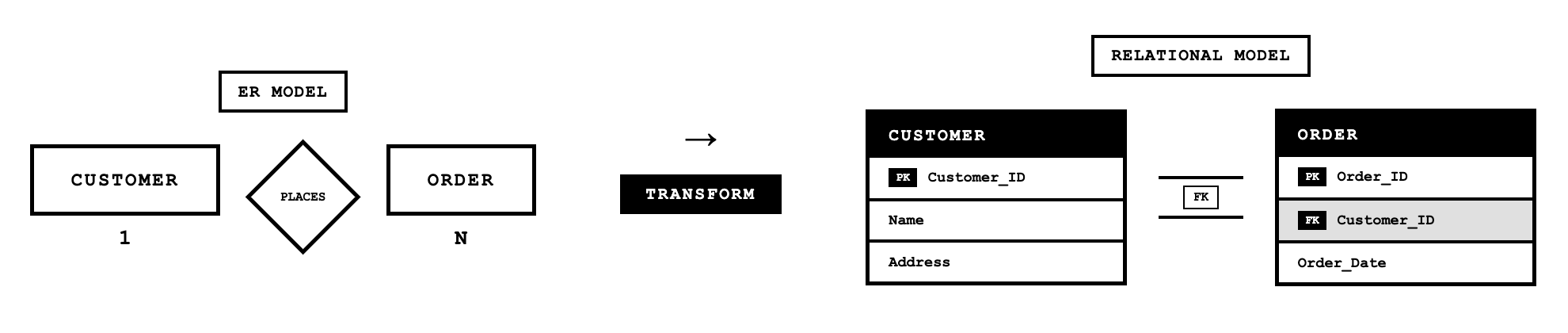
Representing Binary M:N Relationships
Many-to-many relationships require creating a new relation with a composite primary key consisting of the primary keys from both participating entities. Any attributes associated with the relationship become nonkey attributes in this new relation.
Consider a many-to-many relationship between PRODUCT and ORDER, where products can appear on many orders and orders can contain many products. We create an ORDER_LINE relation:
ORDER(Order_Number, Order_Date, Promised_Date)
PRODUCT(Product_ID, Description, Room, City_State_Zip)
ORDER_LINE(Order_Number, Product_ID, Quantity_Ordered)
The composite key (Order_Number, Product_ID) uniquely identifies each line item, and Quantity_Ordered is a nonkey attribute describing that specific product on that specific order.

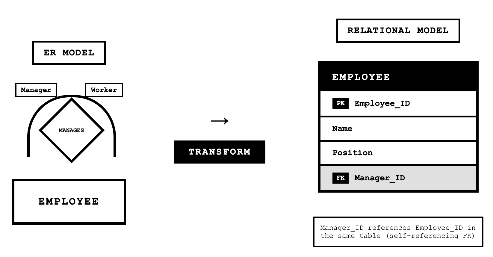
Representing Unary Relationships
Unary relationships, also called recursive relationships, involve a single entity related to itself. For a unary one-to-many relationship, we model this by adding a foreign key to the relation that references the primary key of the same relation. This is called a recursive foreign key.
For example, an EMPLOYEE entity with a "Manages" relationship where one employee manages many other employees becomes:
EMPLOYEE(Employee_ID, Name, Birthdate, Manager_ID)The Manager_ID is a recursive foreign key that references Employee_ID values in the same table.
For unary many-to-many relationships, we create a separate relation with a composite key where both attributes reference the same primary key. For example, a bill-of-materials structure where items contain other items:
ITEM(Item_Number, Name, Cost)
ITEM_BILL(Parent_Item_Number, Component_Item_Number, Quantity)
Both Parent_Item_Number and Component_Item_Number reference Item_Number in the ITEM relation.
View Integration and Merging Relations
View integration is the process of merging normalized relations from separate user views into a consolidated set of well-structured relations. This step is necessary because different users or functional areas often have different perspectives on the same data, and we need to create a single integrated database that serves all needs.
Synonyms
Synonyms occur when two different names are used for the same attribute. For example, one user view might have Student_ID while another has Matriculation_Number, but both refer to the student's identification number. When merging these relations, we must get agreement from users on a single standard name. The merged relation would use one consistent name:
STUDENT(Student_ID, Name, Address)Homonyms
Homonyms occur when a single attribute name is used for different attributes in different contexts. For example, the attribute "Address" might refer to a student's campus address in one view and their permanent home address in another view. When merging, we must create new descriptive names to distinguish them:
STUDENT(Student_ID, Name, Campus_Address, Permanent_Address, Phone_Number)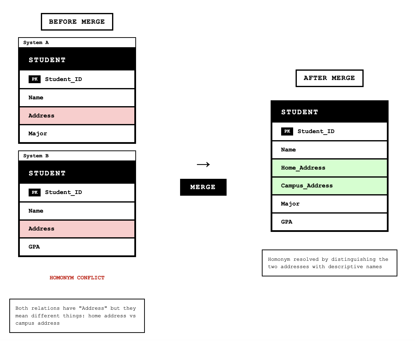
Transitive Dependencies Between Nonkeys
When merging two relations with the same primary key, we might inadvertently create transitive dependencies. Consider merging:
STUDENT1(Student_ID, Major)
STUDENT2(Student_ID, Adviser)
The merged relation would be STUDENT(Student_ID, Major, Adviser). However, if each major has a designated adviser and students are assigned to that adviser, we have a transitive dependency: Student_ID → Major → Adviser. This requires normalizing into:
STUDENT(Student_ID, Major)
MAJOR_ADVISER(Major, Adviser)
Class/Subclass Relationships
Sometimes the merging process reveals class and subclass relationships that weren't explicitly modeled. For example, if we have:
PATIENT1(Patient_ID, Name, Address, Date_Treated)
PATIENT2(Patient_ID, Room_Number)
We might realize that PATIENT can refer to both inpatients and outpatients. This suggests converting to a supertype/subtype structure:
PATIENT(Patient_ID, Name, Address)
INPATIENT(Patient_ID, Room_Number)
OUTPATIENT(Patient_ID, Date_Treated)
Physical Database Design: Fields and Data Types
Physical database design involves making concrete decisions about how data will be stored and accessed. The first decision in physical design is choosing data types for each field. A field is the smallest unit of named application data recognized by system software, and a data type is the coding scheme that the system uses to represent that data.
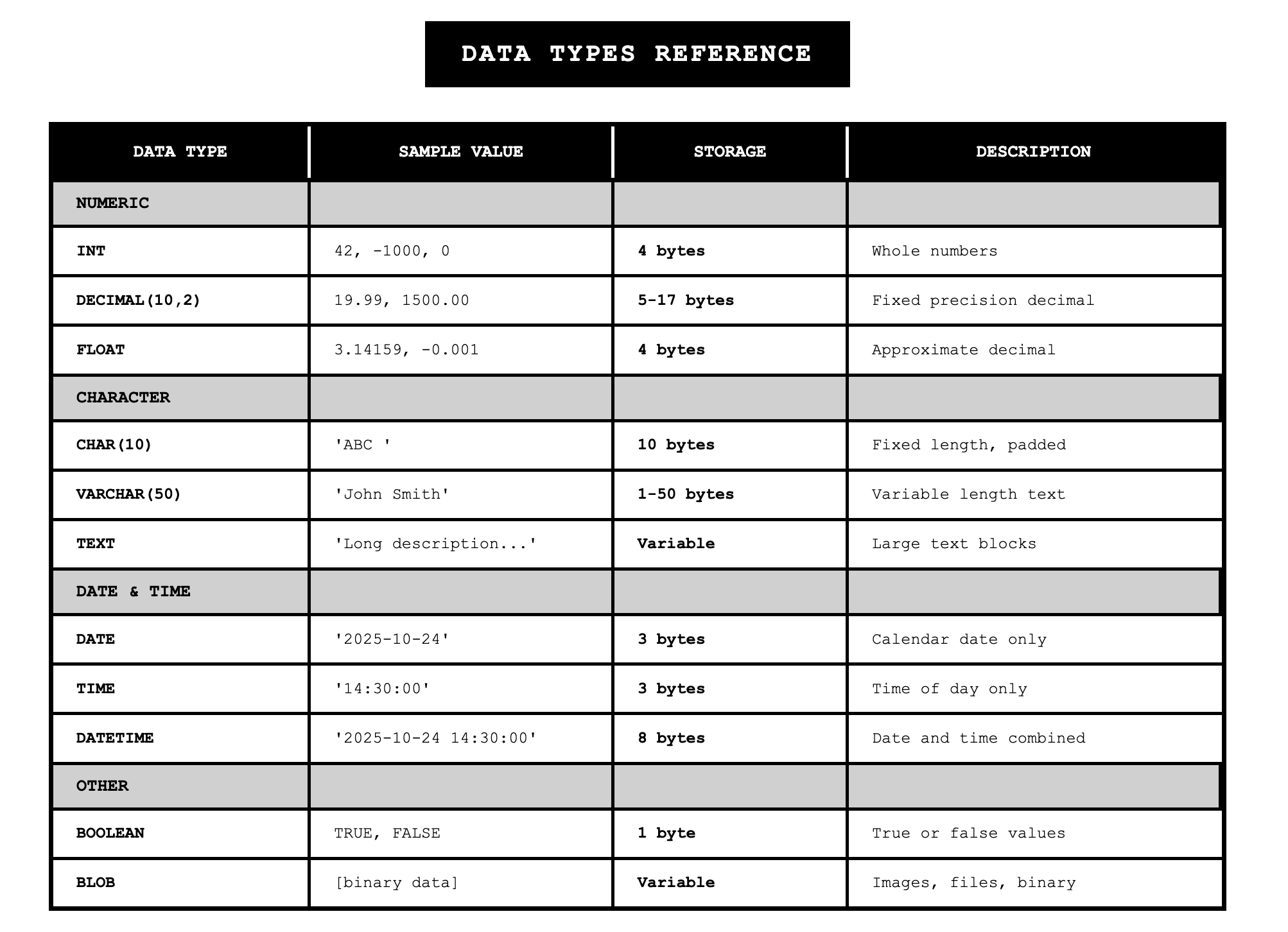
Selecting a data type requires balancing four objectives: minimizing storage space, representing all possible values of the field, improving data integrity for the field, and supporting all data manipulations desired on the field. Different database management systems offer different sets of data types, but common types include:
VARCHAR2 for variable-length character data with a specified maximum length. This type only uses the storage needed for the actual value, making it efficient for fields where the length varies significantly. For example, VARCHAR2(30) can hold up to 30 characters but will only use the space needed for the actual value stored.
CHAR for fixed-length character data. This type always uses the full specified length regardless of the actual value. CHAR(5) always uses five characters of storage, padding with spaces if needed.
NUMBER for numeric values where you can specify precision (total digits) and scale (digits after decimal point). NUMBER(5,2) can hold values from -999.99 to 999.99.
DATE for temporal data that stores century, year, month, day, hour, minute, and second.
BLOB for binary large objects like images, sound clips, or documents that need to be stored as binary data.
Calculated Fields
Calculated fields present a design decision between storing computed values or calculating them on demand. A calculated field is one that can be derived from other database fields. For example, Order_Total might be calculated by summing the price times quantity for all items on an order.
The designer must decide whether to store this calculated value in the ORDER table or compute it whenever needed by summing the ORDER_LINE items. Storing the calculated field provides faster retrieval because the value is already available, but it requires additional storage space and introduces the risk of inconsistency if the value isn't updated properly when underlying data changes. Computing the field on demand saves storage and ensures the value is always current, but it requires computation time for every query that needs the value.
Data Integrity Controls
Physical database design includes implementing controls to ensure data integrity. Default values provide automatic values when no explicit value is entered for a field, reducing data entry errors and ensuring consistent values for commonly used fields.
Range controls limit the values that can be entered into a field. For numeric fields, this might be a minimum and maximum value. For text fields, this might be a list of acceptable values. Range controls prevent obviously invalid data from entering the database.
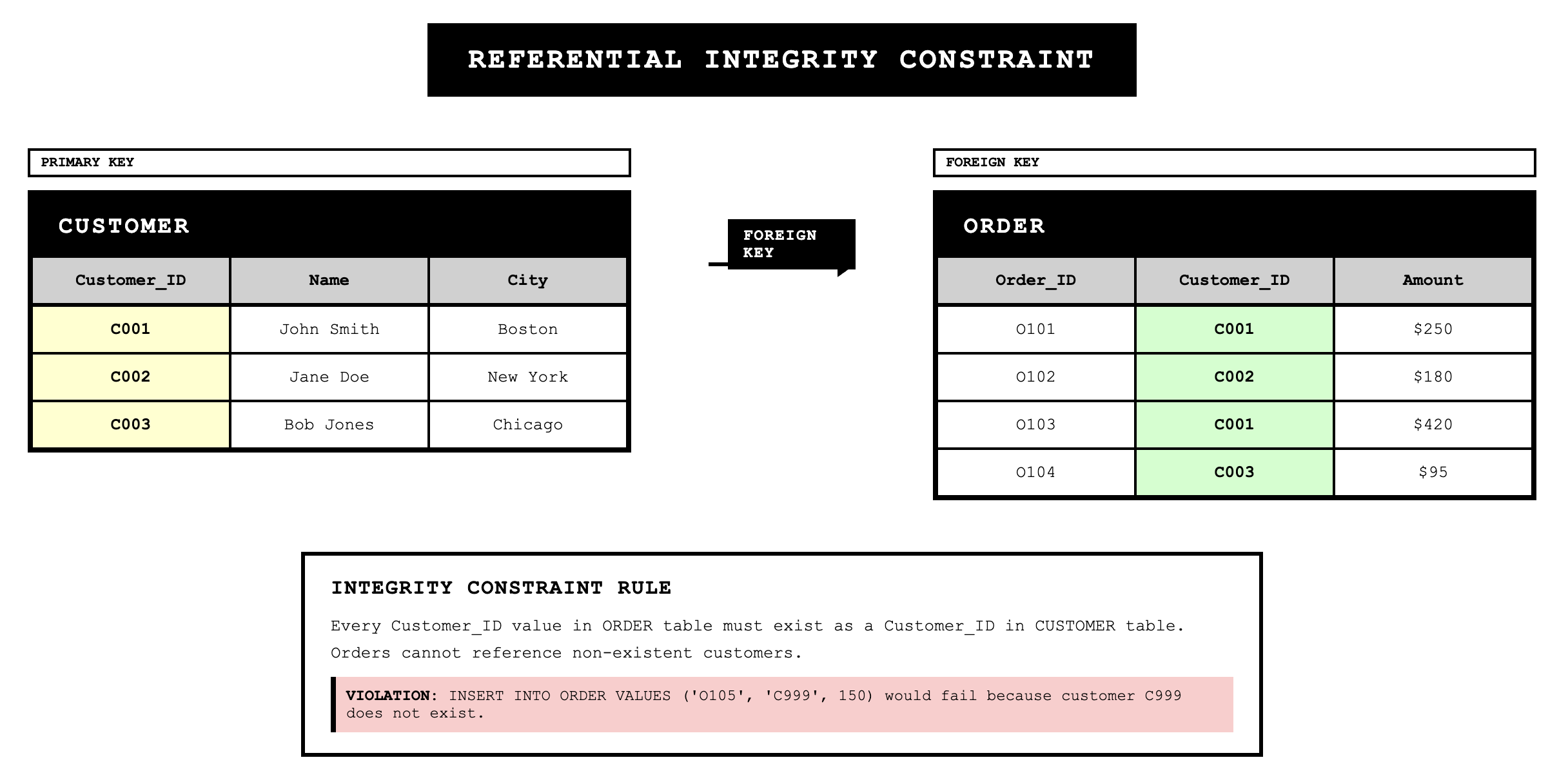
Referential integrity is a rule stating that each foreign key value must match a primary key value in another relation or be null. This constraint prevents orphaned records where a foreign key references a nonexistent primary key. For example, if we have Customer_ID as a foreign key in the ORDER relation, referential integrity ensures that every Customer_ID in ORDER exists in the CUSTOMER relation.
Null values require explicit handling. A null value is distinct from zero, blank, or any other value. It indicates that the value for the field is missing or unknown. Some fields, particularly primary keys and certain foreign keys, should never be null, while other fields might legitimately be null. The database design must specify which fields allow null values and how nulls should be interpreted.
Denormalization and Physical Table Design
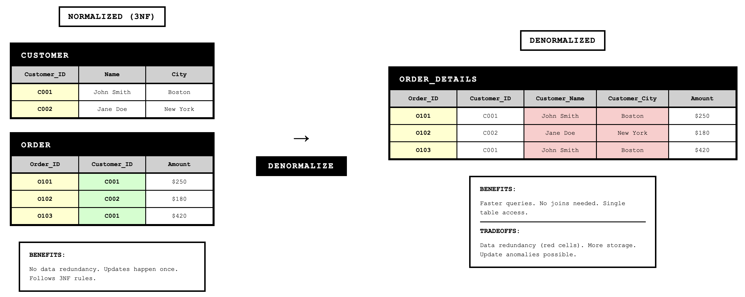
While normalization creates the ideal logical structure, physical database design sometimes requires denormalization to achieve acceptable performance. Denormalization is the process of splitting or combining normalized relations into physical tables based on the affinity of use of rows and fields.
The primary motivation for denormalization is to reduce the number of joins required for common queries. Joining tables is computationally expensive, and queries that join many tables can have poor performance. By combining data from multiple normalized tables into a single physical table, we can eliminate some joins and speed up query execution.
Denormalization by Combining Tables
One common denormalization technique combines two tables with a one-to-one relationship or combines frequently joined tables in one-to-many relationships. For example, if we always retrieve customer data and their account settings together, we might denormalize by combining them into a single table even though they could be normalized as separate entities.
Denormalization by Splitting Tables
Another technique splits a single normalized table into multiple physical tables based on usage patterns. This is called horizontal partitioning or vertical partitioning.
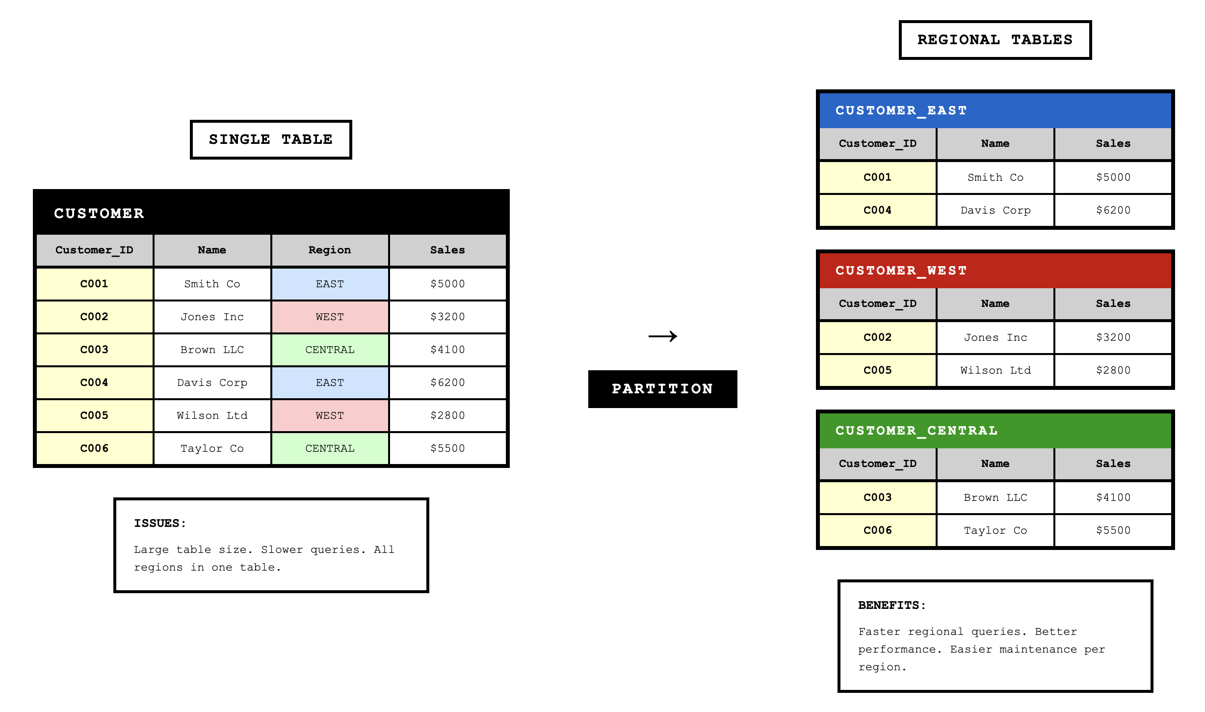
Horizontal partitioning splits rows across multiple tables. For example, we might split a CUSTOMER table into regional tables based on geography. The normalized model has one CUSTOMER relation, but physically we might implement A_CUSTOMER (Atlantic region), P_CUSTOMER (Pacific region), and S_CUSTOMER (Southern region). This speeds up queries that target specific regions because the database only needs to scan the relevant partition.
Vertical partitioning splits columns across multiple tables. If a PRODUCT table has some attributes accessed frequently and others accessed rarely, we might split them. For example, engineering data (Product_ID, Description, Drawing_Number, Weight, Color) might be separated from accounting data (Product_ID, Unit_Cost, Burden_Rate) and marketing data (Product_ID, Description, Color, Price, Product_Manager).
The tradeoff with denormalization is that we reintroduce the possibility of data anomalies that normalization eliminated. Redundant data can become inconsistent if updates aren't properly coordinated. Denormalization should only be used when performance requirements justify accepting these risks.
Table Partitioning
Partitioning is a capability to split a table into separate sections while maintaining a single logical table. Unlike denormalization, partitioning is typically transparent to applications, which still see a single table even though the data is physically distributed.
Range partitioning defines partitions using nonoverlapping ranges of values for a specified attribute. For example, we might partition an ORDER table by Order_Date, with one partition for each year. Queries that filter on date can scan only the relevant partitions.
Hash partitioning assigns rows to partitions using an algorithm that maps attribute values to partition numbers. This distributes data evenly across partitions even when there aren't natural ranges.
Composite partitioning combines both approaches by first segregating data by ranges and then distributing rows within each range using hashing.
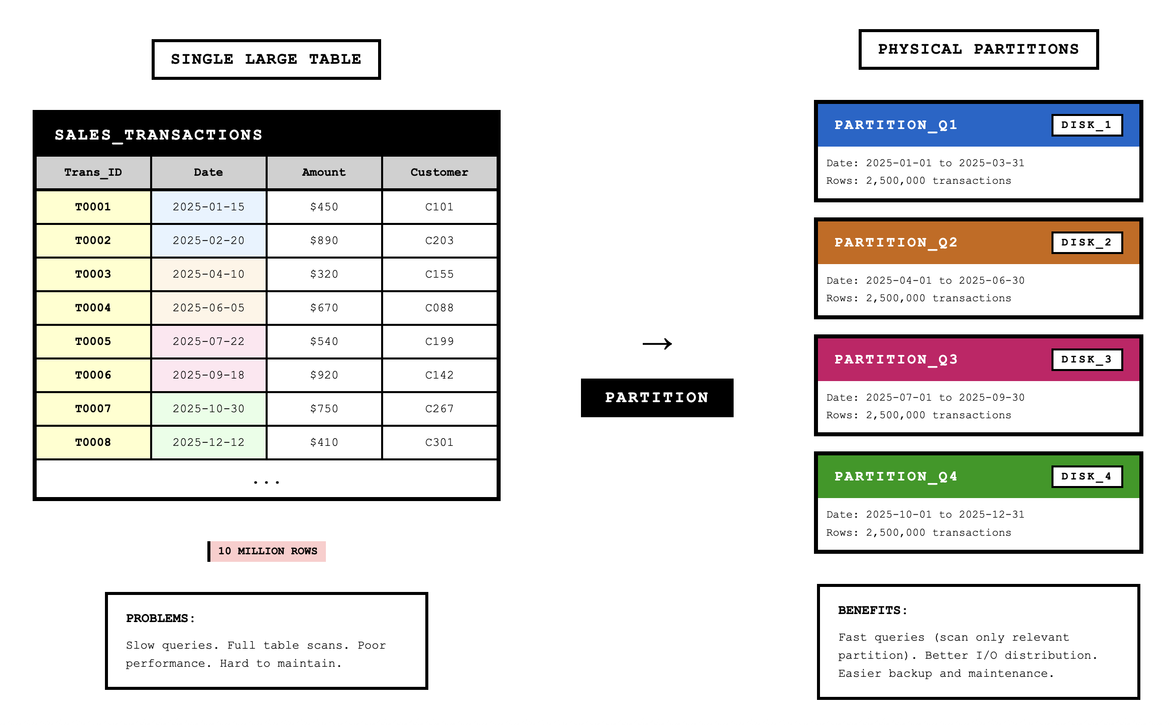
Partitioning improves performance by allowing the database to scan only relevant sections for queries that filter on the partitioning key. It also simplifies maintenance by allowing operations on individual partitions rather than entire tables.
File Organizations
File organization refers to the technique for physically arranging the records of a file. The choice of file organization has major implications for performance. The three basic families of file organization are sequential, indexed, and hashed.
Sequential File Organization
In sequential file organization, rows are stored in sequence according to primary key values. To find a specific row, the database must scan from the beginning of the file until it finds the target row. Sequential organization provides very fast sequential retrieval when processing all rows in key order, but it makes random retrieval of individual rows impractical. Adding, deleting, or updating rows often requires rewriting the entire file.

Indexed File Organization
Indexed file organization maintains rows (either sequentially or non-sequentially) and creates an index that maps key values to row locations. An index is a table that contains key values and pointers to where those rows are stored. When searching for a specific key value, the database searches the index to find the pointer, then follows the pointer directly to the row location.
Indexed organization supports both sequential retrieval (by scanning through the index in order) and random retrieval (by searching the index for specific values). The main disadvantage is the extra storage space required for indexes and the extra time to maintain indexes when data changes.

Indexes can be created on any field, not just primary keys. A secondary key is an attribute or combination of attributes for which more than one row may have the same value. Secondary key indexes allow fast retrieval based on non-unique values. For example, an index on Customer_Name allows fast retrieval of all customers with a particular name, even though names aren't unique.
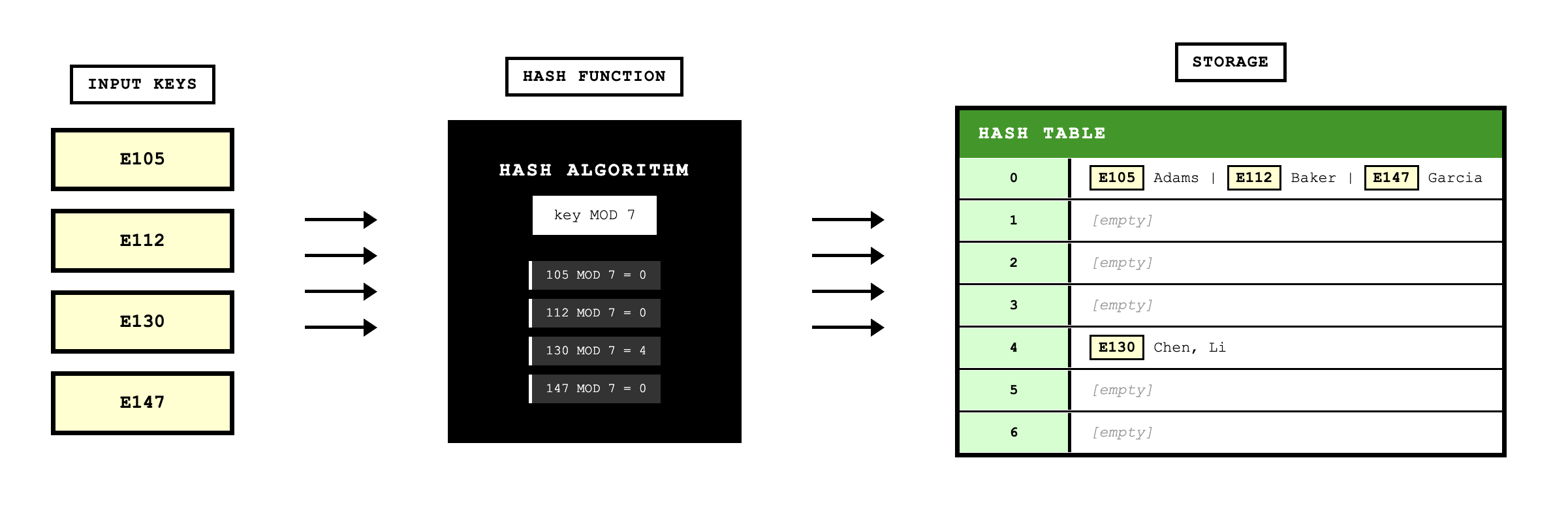
Hashed File Organization
Hashed file organization uses an algorithm to compute the storage address for each row from the primary key value. When inserting a row, the algorithm transforms the key value into a storage address. When retrieving a row, the same algorithm computes where the row should be located. This provides very fast random retrieval but makes sequential retrieval impractical because rows aren't stored in key order.
Comparing File Organizations
Each file organization optimizes different operations. Sequential organization is best for processing all rows in order but poor for random access. Indexed organization handles both sequential and random access moderately well and supports multiple key retrieval through multiple indexes. Hashed organization provides the fastest random access but doesn't support sequential retrieval or multiple key access.

Designing Indexes
Choosing which fields to index involves tradeoffs between query performance and update performance. Each index speeds up certain queries but slows down inserts, updates, and deletes because the index must be maintained.
The guidelines for index selection include specifying a unique index for the primary key of each table, which most database systems do automatically. We should also specify indexes for foreign keys because these are frequently used in joins. Finally, we should create indexes for nonkey fields that are referenced in WHERE clauses, ORDER BY clauses, or GROUP BY clauses for queries that will be executed frequently.
However, we should avoid creating too many indexes. Each additional index consumes storage space and slows down modification operations. The decision requires analyzing the query patterns and update frequencies for the specific application.
File Controls: Backup and Security
Physical database design must address protection from failure and security from unauthorized use. These goals are achieved through backup procedures and security controls.
Backup techniques for file restoration include periodically making complete backup copies of files, storing each change in a transaction log or audit trail, and maintaining before-images or after-images of rows as they're modified. These techniques allow the database to be restored to a consistent state after hardware failures, software errors, or user mistakes.
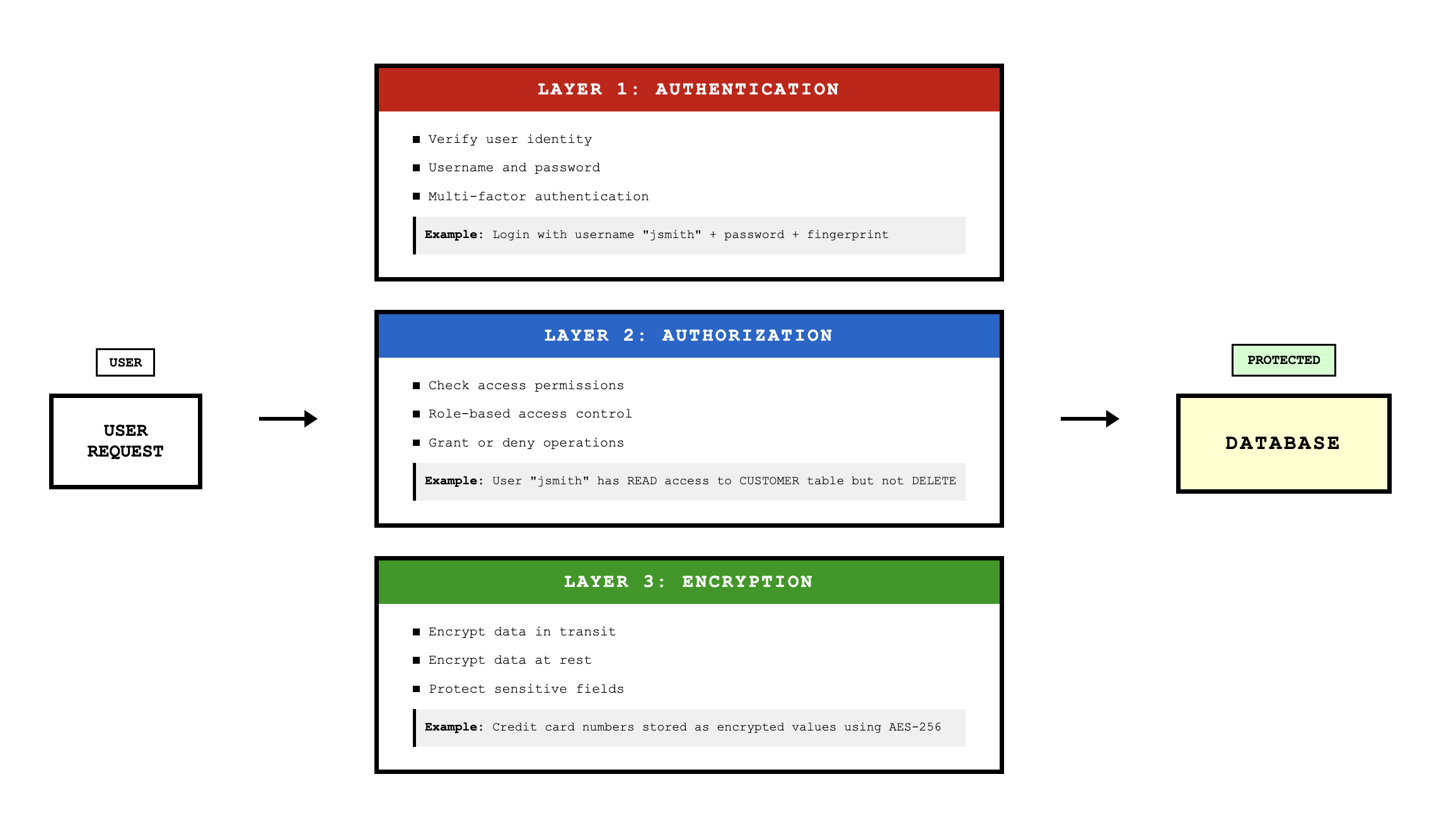
Security controls restrict access to authorized users and limit what they can do. Encryption protects data by encoding it so that it's unreadable without the decryption key. User authentication requires users to identify themselves through usernames and passwords or other credentials. Authorization controls specify what operations each user can perform on which data. Many systems force users to work with views or copies of data rather than directly manipulating the actual tables, providing an additional layer of protection.
Conclusion
Database design transforms conceptual models into implementable structures through a systematic process. Logical design focuses on creating normalized relations that eliminate redundancy and prevent anomalies. We apply normalization rules to ensure each relation is well-structured, with attributes depending properly on primary keys. We transform entity-relationship diagrams into relations following standard patterns based on entity types and relationship cardinalities. We merge relations from different user views while resolving synonyms, homonyms, and hidden dependencies.
Physical design makes concrete decisions about storage and access mechanisms. We choose data types that balance storage efficiency with data representation requirements. We implement field-level controls including defaults, range checks, and null handling. We decide whether to store or compute calculated fields. We sometimes denormalize relations to improve performance, accepting the risk of anomalies in exchange for faster queries. We partition large tables to improve both performance and maintainability.
File organization and indexing decisions determine how efficiently the database can retrieve and update data. Sequential organization optimizes sequential processing. Indexed organization balances sequential and random access. Hashed organization optimizes random retrieval. Indexes speed up queries at the cost of storage and update overhead, requiring careful analysis of query patterns to choose which fields to index.
Finally, we implement controls for backup and security to protect data from loss and unauthorized access. The complete database design provides both the logical correctness of normalized structures and the physical efficiency needed for actual applications.